Kronecker Product


The Kronecker Product is a snazzy bit of linear algebra that I don’t use often enough to remember exactly how it works. I have most recently run in to it during an excellent course on machine learning using Spark MLlib. There it was used to simplify a variety of data set feature samplings (e.g. grouped offsets within a time series, aggregate blocks in a series). I have also used it in previous data science flavored courses.

warning: may be slow to render the mathy bits while mathjax loads

The first example in the course lab material was straight forward enough:
$$ \begin{bmatrix} 1 & 2 \\\ 3 & 4 \end{bmatrix} \otimes \begin{bmatrix} 1 & 2 \end{bmatrix} = \begin{bmatrix} 1 \cdot 1 & 1 \cdot 2 & 2 \cdot 1 & 2 \cdot 2 \\\ 3 \cdot 1 & 3 \cdot 2 & 4 \cdot 1 & 4 \cdot 2 \end{bmatrix} = \begin{bmatrix} 1 & 2 & 2 & 4 \\\ 3 & 6 & 4 & 8 \end{bmatrix} $$
But the second example starts to get obscure:
$$ \begin{bmatrix} 1 & 2 \\\ 3 & 4 \end{bmatrix} \otimes \begin{bmatrix} 1 & 2 \\\ 3 & 4 \end{bmatrix} = \begin{bmatrix} 1 \cdot 1 & 1 \cdot 2 & 2 \cdot 1 & 2 \cdot 2 \\\ 1 \cdot 3 & 1 \cdot 4 & 2 \cdot 3 & 2 \cdot 4 \\\ 3 \cdot 1 & 3 \cdot 2 & 4 \cdot 1 & 4 \cdot 2 \\\ 3 \cdot 3 & 3 \cdot 4 & 4 \cdot 3 & 4 \cdot 4 \end{bmatrix} = \begin{bmatrix} 1 & 2 & 2 & 4 \\\ 3 & 4 & 6 & 8 \\\ 3 & 6 & 4 & 8 \\\ 9 & 12 & 12 & 16 \end{bmatrix} $$
Using the same values in each input matrix makes it confusing as to what operand has come from where. This would be so much clearer to me if unique numbers were used for the inputs:
$$ \begin{bmatrix} 1 & 2 \\\ 3 & 4 \end{bmatrix} \otimes \begin{bmatrix} 5 & 6 \\\ 7 & 8 \end{bmatrix} = \begin{bmatrix} 1 \cdot 5 & 1 \cdot 6 & 2 \cdot 5 & 2 \cdot 6 \\\ 1 \cdot 7 & 1 \cdot 8 & 2 \cdot 7 & 2 \cdot 8 \\\ 3 \cdot 5 & 3 \cdot 6 & 4 \cdot 5 & 4 \cdot 6 \\\ 3 \cdot 7 & 3 \cdot 8 & 4 \cdot 7 & 4 \cdot 8 \end{bmatrix} = \begin{bmatrix} 5 & 6 & 10 & 12 \\\ 7 & 8 & 14 & 16 \\\ 15 & 18 & 20 & 24 \\\ 21 & 24 & 28 & 32 \end{bmatrix} $$
Which is the approach used on the Kronecker Wikipedia page. But I still want to see this more clearly and without needing to be shown the intermediate computations:
$$ \begin{bmatrix} 1 & 0 & 0 \\\ 0 & 1 & 0 \\\ 0 & 0 & 1 \end{bmatrix} \otimes \begin{bmatrix} 1 & 2 \\\ 3 & 4 \end{bmatrix} = \begin{bmatrix} 1 & 2 & 0 & 0 & 0 & 0 \\\ 3 & 4 & 0 & 0 & 0 & 0 \\\ 0 & 0 & 1 & 2 & 0 & 0 \\\ 0 & 0 & 3 & 4 & 0 & 0 \\\ 0 & 0 & 0 & 0 & 1 & 2 \\\ 0 & 0 & 0 & 0 & 3 & 4 \end{bmatrix} $$
Hey, look at how that 1-2-3-4 block gets replicated! But what about all those multiplications? OK, try this:
$$ \begin{bmatrix} 1 & 0 & 0 \\\ 0 & 5 & 0 \\\ 0 & 0 & 10 \end{bmatrix} \otimes \begin{bmatrix} 1 & 2 \\\ 3 & 4 \end{bmatrix} = \begin{bmatrix} 1 & 2 & 0 & 0 & 0 & 0 \\\ 3 & 4 & 0 & 0 & 0 & 0 \\\ 0 & 0 & 5 & 10 & 0 & 0 \\\ 0 & 0 & 15 & 20 & 0 & 0 \\\ 0 & 0 & 0 & 0 & 10 & 20 \\\ 0 & 0 & 0 & 0 & 30 & 40 \end{bmatrix} $$

In Python’s numpy the function is named kron. In R it is named kronecker and %x% can be used in place of the full name (in keeping with R’s tradition of being weird).

Learning Deep Learning

Learning about Deep Learning that is.

It’s a specialized area of neural networks which itself is a specialized area of machine learning. Deep Learning is hot right now with very impressive results on tasks which have been difficult for other machine learning methods to solve.

I need to learn more and now. But how? Over the last few years the rise of the MOOCs has been providing a rich stream of learning possibilities for a huge range of subjects including high end tech as in Andrew Ng’s Coursera Machine Learning class, where basic neural networks were covered as part of the course.

Currently there is no Deep Learning MOOC. This will need to be a self-constructed curriculum. Who are the leaders in the field? The University of Toronto’s Geoffrey Hinton is on top, very closely followed by Yann LeCun of NYU and Yoshua Bengio at the University of Montreal. Last year Hinton was hired by Google and LeCun was hired by Facebook. Both retain their academic positions and part time teaching responsibility.

That’s the background. The rest of this post describes my start on learning about Deep Learning. The journey is far from over. These are only my initial steps and a few thoughts about where to go next.

Hinton’s Coursera Neural Networks class was offered in October 2012. It is an advanced neural networks class that goes way beyond the simple nets covered in Ng’s course. It is not specifically a deep learning class but does spend several lectures on the topic. The course has not been offered again and I don’t think it will. Hinton must be very busy with Google and indicates on his web page that he is not accepting new students for graduate study.

I looked at some of the archived video from this class. Even after Ng’s class I did not feel like I had the background to really appreciate the material. These lectures get deep fast. I need to prepare. Also for my particular learning style I want the “50,000 foot view” for Deep Learning and a sense of where all the pieces are going to fit.

So instead of jumping right in to the nearly 13 hours of Coursera class video I found A Tutorial on Deep Learning Hinton presented in 2009. The tutorial runs 3 hours and felt deeper than what I needed at that point. It may have been my unfamiliarity with Hinton’s
presentation style or maybe he was trying to compress the entirety of his experience to fit the venue. I did not finish watching this one.

Along the way I found Hugo Larochelle’s Neural Networks class videos. This is not a MOOC, just the videos from the course he teaches at Université de Sherbrooke. I like the presentation style and find the material accessible. He covers many neural network topics well beyond the basics. Still this is over 16 hours of lectures! I am impatient to get further in to deep learning concepts so I’ve been cherry picking these. I’ve watched most of the first two units to “calibrate” with what I learned from Ng’s class and have also gone through most of the autoencoder material.

Next I came upon a LeCun and Bengio lecture I could really get my mind around. It’s the one hour 2009 ICML workshop Tutorial: Deep Learning Architectures. Digging further I found LeCun’s 2013 ICML Deep Learning Tutorial very useful. This one is 1½ hours long. Now after watching these two I’m starting to see the shape of the field, that 50,000 foot view. This is what I need for my learning style, everyone’s style is different.

Will Stanton’s presentation at the May 2014 Data Science & Business Analytics meetup confirmed many of my perceptions, corrected some others, and exposed new dimensions to investigate.

Immediately after that I found a talk by Jeremy Howard at the Data Science Melbourne meetup on May 12th, 1¾ hours. (Jeremy was enrolled as a student in the initial offering of Bill Howe’s Coursera Introduction to Data Science. He contributed to many interesting forum threads there. He is currently involved in a startup creating deep learning tools. His last position was as president and chief scientist at Kaggle.) This talk is excellent. Jeremy covers the emergence of deep learning over other techniques, social and economic implications, and a bit of implementation detail. This is a must-watch, the talk that I would have liked to start with, but it did not yet exist.

Now at this point I am finally ready to absorb some Hinton presentations. His Google Tech Talks Recent Developments in Deep Learning (2010) and The Next Generation of Neural Networks (2007) were very good even if I did watch them out of chronological order. Each talk is one hour.

What next?

  • Working through the neural network course videos from both Hinton and Larochelle.
  • Trying out open source deep learning software packages.
  • Continuing to search/watch lectures. They are not all on youtube.
  • Google+ communities Machine Learning and Deep Learning are both very active.
  • Reddit has a very active and interesting subreddit /r/machinelearning. Yann LeCun did an AMA there last month. (There is also a /r/deeplearning subreddit but nothing is happening there.)
  • Check out LeCun’s Spring 2014 NYU Deep Learning course videos and notes.

GPU Shopping

GPUSo you want to run some deep learning code and heard you need a GPU? This seems correct. For deep learning problems of sufficient size to be interesting the alternative is to either (A) use a supercomputer or (B) have your body cryogenically preserved and arrange to be reanimated when your program completes. The second option makes iterative development cumbersome.

You could also rent time on a GPU equipped cloud instance. But I believe this only makes sense with both already-debugged code and the appropriate economics. A recent deep learning success story reported that two GPUs were used over a week long training period. At the current AWS rate this would cost about $220 for that single run.

Which GPU Vendor?

Nvidia. That’s it. Nvidia has been very active in promoting their CUDA programming model. There are online courses available for CUDA and a variety of development tools. Local development will be the way to go for creating new code. The OpenCL programming model is an alternative for GPU use but it does not have the fine grained device control necessary to take maximum advantage of the hardware. Current versions of Theano, Torch, and other machine learning libraries work with CUDA, not OpenCL.

I have not been motivated to understand why, but it seems that bitcoin miners prefer the AMD/ATI GPU family over Nvidia for their code. But that’s bitmining not deep learning.

Which Card?

How much do you want to spend? At the lower end $100 will buy a GTX 750. This card has 512 compute cores but is only available with 1GB of memory. This seems like it will run out of space on machine learning tasks very quickly. In the $130 – $150 range the 640 core, 2GB, GTX 750 Ti looks like a much better choice. Both of these cards are based on Nvidia’s latest “Maxwell” processors and have much lower power requirements than earlier cards.

A step up to the $380 – $400 range will buy a 1536 core, 4GB, GTX 770. This is the same level of GPU muscle available through AWS cloud instances. At the top of the range you can be really crazy and get the Titan-Z with 5760 cores and 12GB of memory for $3000.

If the purchase can wait until late 2014 the Maxwell architecture is supposed to be moving in to the mid and high end cards. So cooler, quieter, and less need for a high wattage power supply.

Maybe an older card to save a few bucks? Maybe, but the “compute capability” evolves as the generations of GPUs move forward. Check the charts on the CUDA Wikipedia page to see what compute capability goes with a specific GPU. I recently saw a low end GT 640 for a good price. That seemed like a nice starter for some at-home CUDA coding. However further investigation revealed the card I was considering had slower GDDR3 memory and a lower compute capability compared to other GT 640s with GDDR5. Not such a good deal after all.

Where Will You Plug It In?

Now the decision gets complicated. First understand that moving data between the GPU and the computer’s main memory is going to be done a LOT. This and coordination overhead will take up most of the time spent on the “GPU computing” portion of processing. Even though there may be 1500+ computing cores available on a GPU they cannot all be kept busy all the time. You will actually be doing quite well if the GPU-aware parts of your problem run 50x to 100x faster than a CPU-only version of the code. It will help if GPU/CPU data transfers occur less frequently by having enough GPU memory to keep data on-board avoiding repeated back and forth shuffling. It is also important the transfers that do occur are as fast as possible.

Most of these cards are designed to go in a PCIe 3.0 motherboard slot. Will it work in PCIe 2.0 slots? It should, but data transfer rates are 2x faster for the 3.0 slots. The article Theoretical vs. Actual Bandwidth: PCI Express and Thunderbolt gets a lot deeper in to 2.0 vs 3.0 difference and “lanes” (the Thunderbolt stuff does not apply here). But their performance summary conclusions are for game image rendering and not machine learning computation.

Oh, and where did you plan to plug in your monitor? I’m not sure what fraction of a GPU would be consumed by the OS user interface, but it can’t be good for running machine learning tasks at full speed. So what about that UI then? Two choices, both require a relatively modern motherboard. If your CPU can handle graphics directly (recent Intel and the AMD APU series), problem solved. Or if you have another dedicated GPU for graphics you will need an additional PCIe slot for that. Just watch out for the “lane restrictions” with multiple PCIe devices. For instance some mobos will use x16 lane connections to a single GPU but plug in a second GPU and they each get x8 lanes. One possibility (I have not actually tested) would have the shiny new GPU for machine learning tasks in a PCIe 3.0 slot and a less capable GPU dedicated to the user interface in a PCIe 2.0 slot.

Need to play Call of Duty, Watch Dogs, or GTA using your hottest GPU? Better get used to reconfiguring displays and swapping cables.

PyCon 2014 Videos

The 2014 PyCon in Montreal is over and 138 videos from the conference have already been posted. There are a huge variety of topics covered. To avoid scrolling through the entire list every time I want to see what I missed by staying home here is a subset of session and tutorial videos of interest to data science and machine learning fans. I have listed running times as h:mm:ss. Summary text is from the pyvideo.org site.

Sessions (short)

Diving into Open Data with IPython Notebook & Pandas, 0:30:55
I’ll walk you through Python’s best tools for getting a grip on data: IPython Notebook and pandas. I’ll show you how to read in data, clean it up, graph it, and draw some conclusions, using some open data about the number of cyclists on Montréal’s bike paths as an example.

Know Thy Neighbor: Scikit and the K-Nearest Neighbor Algorithm, 0:20:56
One of the great features of Python is its machine learning capabilities. Scikit is a rich Python package which allows developers to create predictive apps. In this presentation, we will guess what type of music do Python programmers like to listen to, using Scikit and the k-nearest neighbor algorithm.

Enough Machine Learning to Make Hacker News Readable Again, 0:28:49
It’s inevitable that online communities will change, and that we’ll remember the community with a fondness that likely doesn’t accurately reflect the former reality. We’ll explore how we can take a set of articles from an online community and winnow out the stuff we feel is unworthy. We’ll explore some of the machine learning tools that are just a “pip install” away, such as scikit-learn and nltk.

How to Get Started with Machine Learning, 0:25:50
Provide an introduction to machine learning to clarify what it is, what it’s not and how it fits into this picture of all the hot topics around data analytics and big data.

Realtime predictive analytics using scikit-learn & RabbitMQ, 0:28:58
scikit-learn is an awesome tool allowing developers with little or no machine learning knowledge to predict the future! But once you’ve trained a scikit-learn algorithm, what now? In this talk, I describe how to deploy a predictive model in a production environment using scikit-learn and RabbitMQ. You’ll see a realtime content classification system to demonstrate this design.

Tutorials (long)

Mining Social Web APIs with IPython Notebook, 3:25:24
Social websites such as Twitter, Facebook, LinkedIn, Google+, and GitHub have vast amounts of valuable insights lurking just beneath the surface, and this workshop minimizes the barriers to exploring and mining this valuable data by presenting turn-key examples from the thoroughly revised 2nd Edition of Mining the Social Web.

Bayesian statistics made simple, 3:15:29
An introduction to Bayesian statistics using Python. Bayesian statistics are usually presented mathematically, but many of the ideas are easier to understand computationally. People who know Python can get started quickly and use Bayesian analysis to solve real problems. This tutorial is based on material and case studies from Think Bayes (O’Reilly Media).

Beyond Defaults: Creating Polished Visualizations Using Matplotlib, 3:08:23
When people hear of matplotlib, they think rudimentary graphs that will need to be touched up in photoshop. This tutorial aims to teach attendees how to exploit the functionality provided by various matplotlib libraries to create professional looking data visualizations.

Data Wrangling for Kaggle Data Science Competitions — An etude, 3:22:04
Let us mix Python analytics tools, add a dash of Machine Learning Algorithmics & work on Data Science Analytics competitions hosted by Kaggle. This tutorial introduces the intersection of Data, Inference & Machine Learning, structured in a progressive mode, so that the attendees learn by hands-on wrangling with data for interesting inferences using scikit-learn (scipy, numpy) & pandas

Hands-on with Pydata: how to build a minimal recommendation engine, 3:21:00
In this tutorial we’ll set ourselves the goal of building a minimal recommendation engine, and in the process learn about Python’s excellent Pydata and related projects and tools: NumPy, pandas, and the IPython Notebook.

Python for Social Scientists, 3:27:00
Many provocative social questions can be answered with data, and datasets are more available than ever. Start working with it here. First we’ll download and visualize one data set from the World Bank Indicators page together, using Matplotlib. Then you’ll have time on your own to pick another data set from any online source and plot that. At the end every person/pair will share what they found.

Exploring Machine Learning with Scikit-learn, 3:24:14
This tutorial will offer an introduction to the core concepts of machine learning, and how they can be easily applied in Python using Scikit-learn. We will use the scikit-learn API to introduce and explore the basic categories of machine learning problems, related topics such as feature selection and model validation, and the application of these tools to real-world data sets.

Diving deeper into Machine Learning with Scikit-learn, 3:15:13
This tutorial session is an hands-on workshop on applied Machine Learning with the scikit-learn library. We will dive deeper into scikit-learn model evaluation and automated parameter tuning. We will also study how to scale text classification models for sentiment analysis or spam detection and use IPython.parallel to leverage multi-CPU or ad-hoc cloud clusters.

Machine Learning Madness

B-ball is next month but it looks like the University of Colorado Computer Science Department has picked a different theme for February. The colloquium schedule has Mark Schmidt presenting Opening up the Optimization Black-Box for Large-Scale Machine Learning on 2/18. The following week has Bert Huang on Structured Machine Learning for the Complex World, 2/25, and Tianbao Yang presents Optimization in Machine Learning: Algorithms, Theories and Applications on 2/27.

CU event links may expire soon after the event occurs. See the current colloquium schedule here anytime. Past events are available on the department’s vimeo channel.

Andrew, Jeremy, and PayPal

techXploration

Yes, PayPal! They host TechXploration, a monthly meetup in San Jose. Andrew Ng spoke on deep learning in August 2013. Youtube links to his presentation can be found in the meetup comments and also are repeated here.
part 1 (14:32), part 2 (14:37), part 3 (14:54), part 4 (12:09), part 5 (14:38), part 6 (5:41)

Also of interest: Jeremy Howard, Chief Data Scientist and President at Kaggle, spoke in July 2013.
part 1 (19:14), part 2 (19:33), part 3 (14:00), part 4 (17:17)

Debugging Optimizer Failure – Not

Kaggle Digit Recognizer series

KdigitsSee9watFrom yesterday’s post:

Octave appears to be failing on the first iteration inside the fmincg() optimization function. The error message is not very helpful. It complains of being out of memory or an index exceeding its range. No line number given.

I could not reproduce this failure. This was on a “fresh” run of Octave so perhaps it was caused by some weird program state left over from ongoing development. Note to self: try restarting Octave when mysterious crashes with unhelpful error messages occur.

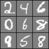
So then before the science begins let’s try one more Kaggle submission, this time using all 42,000 samples to train the neural network. Same as last attempt are the 350 and 100 node hidden layers, lambda 1, and 500 training iterations. Run time was about 5000 seconds (1 hour, 13 minutes), final cost function 0.0671, and self-classified accuracy 99.714%.KdigitsSubmit-4

Slight improvement but probably not meaningful. There is so much random stuff going on here, from the random initialization of Thetas, to whatever random selection is done at Kaggle in scoring the results. The cross validation and analysis discussed at the end of yesterday’s post really are next.

Adding a Second Hidden Layer

Kaggle Digit Recognizer series

KdigitsSee9The initial results (previous post) for the digit classifier were coming in with an accuracy 4 points below the Kaggle-provided sample solutions. This was with only two naive attempts. First was a neural net with a 25-node hidden layer trained over 50 iterations. Next was a net with a 300-node hidden layer trained for 5000 iterations. Some improvement may be gained by tuning the regularization lambda. However no training data subsetting and cross validation has been done yet towards this goal.

It seemed reasonable (and interesting!) to modify the code to allow a second hidden node layer in pursuit of better results. Where to start? The new code will be cloned from what is already working. The single hidden layer functions will remain intact to allow easy side-by-side testing of solutions. The cost function clearly needs to change so nnCostFunction2H() will be used for that. I’m adopting a 2H suffix for functions which support the dual hidden layer network model.

I like the confidence that comes from checking the cost function’s gradients against computed numerical gradients so there will be a checkNNGradients2H() as well.

A predict2H() will be needed too. It would be preferable to have all the training and test data prediction code together in a single function. But at this point in development I would rather have the single and dual hidden layer top level orchestration code in separate files to avoid if-then toxemia in getting all the bits right. Therefore we’ll have trainNN2H.m and runNN2H.m as top level scripts for training the net and producing predicted classifications for submission to Kaggle.

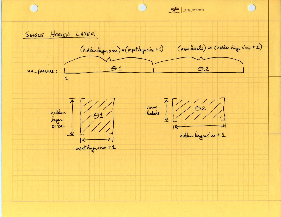
So the changes are really not that extensive. They must be precise though, no room to get sloppy if the vectorized code is expected to work properly. The part of the existing code that was bothering me most deals with reconstructing the Theta matrices. I think there is too much math going on as parameters to the reshape() function calls. I find code like this hard to read and frightening to consider extending:

% Obtain Theta1 and Theta2 back from nn_params
Theta1 = reshape(nn_params(1:hidden_layer_size * (input_layer_size + 1)), ...
                 hidden_layer_size, (input_layer_size + 1));

Theta2 = reshape(nn_params((1 + (hidden_layer_size * (input_layer_size + 1))):end), ...
                 num_labels, (hidden_layer_size + 1));

I need a picture of what is happening here!
singlehiddenlayer

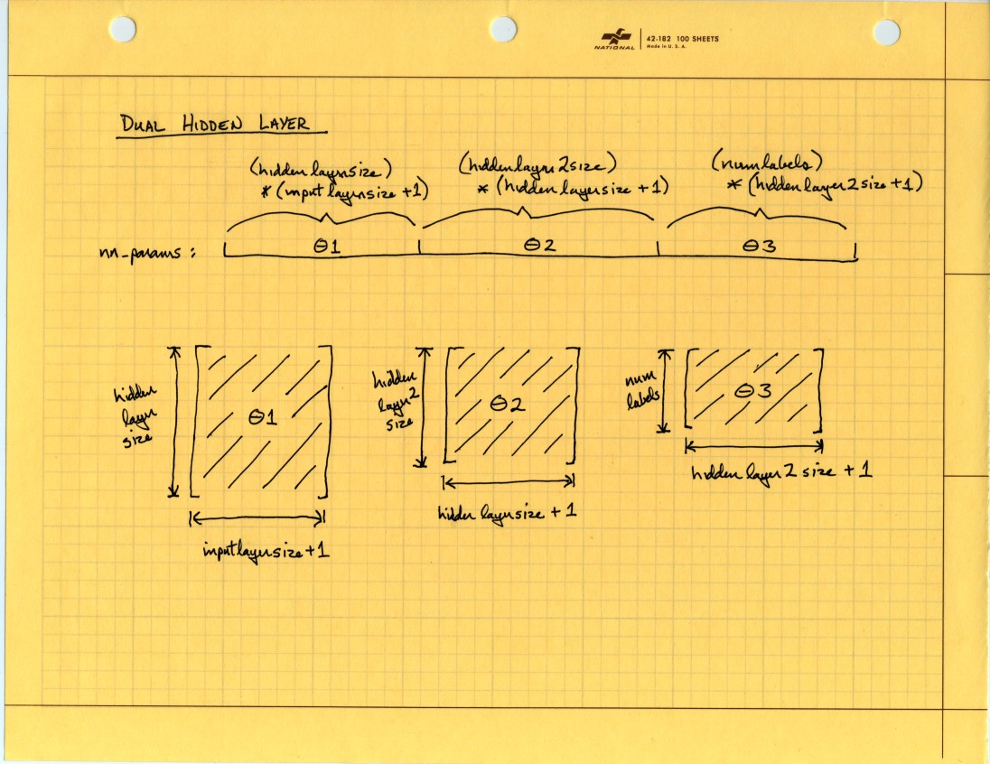
So then for two hidden layers Theta recovery will look like this:
dualhiddenlayer

And from that picture I can see a pattern of how the Theta dimensions progress giving me a pretty good idea how to proceed if I want to parameterize the hidden layer depth. Also, the Theta recovery is done in at least two places in the existing code so I’ve replaced it with a function:

function [Theta1 Theta2 Theta3] = reshapeTheta2H(nn_params, ...
                                                 input_layer_size, ...
                                                 hidden_layer_size, ...
                                                 hidden_layer2_size, ...
                                                 num_labels)
%reshapeTheta2H Recovers Theta matrices for 2 hidden layer NN from flattened vector

    Theta1_size = hidden_layer_size * (input_layer_size + 1);
    Theta2_size = hidden_layer2_size * (hidden_layer_size + 1);
    Theta3_size = num_labels * (hidden_layer2_size + 1);

    Theta1_start = 1;
    Theta2_start = Theta1_size + 1;
    Theta3_start = Theta1_size + Theta2_size + 1;

    Theta1 = reshape(nn_params(Theta1_start : Theta1_size), ...
                     hidden_layer_size, (input_layer_size + 1));

    Theta2 = reshape(nn_params(Theta2_start : (Theta1_size + Theta2_size)), ...
                     hidden_layer2_size, (hidden_layer_size + 1));

    Theta3 = reshape(nn_params(Theta3_start : end), ...
                     num_labels, (hidden_layer2_size + 1));

end

Now another naive test run, no regularization tuning yet. This neural net will use 350 nodes in the first hidden layer, 100 nodes in the second hidden layer, lambda = 1, and 500 training iterations. The full training set of 42,000 samples will be used.

But no! Octave appears to be failing on the first iteration inside the fmincg() optimization function. The error message is not very helpful. It complains of being out of memory or an index exceeding its range. No line number given. This needs investigation but not right now, I’d really like to see some results.

Cutting down the training set size by 20% to 33,600 samples works with no complaints. Run time is just under 3600 seconds (1 hour). Final iteration (500) cost function value is 0.0596 and self-classified accuracy is 99.821%. The Kaggle submission for this net scored 96.486% accuracy.
KdigitsSubmit-3

That is an improvement, but not so much. It is still under the Kaggle sample solution performance but getting closer. Now it’s time to put the science in Data Science. Next to-do is cross validation to find a proper lambda. And next after that will be examining training vs cross validation error rates over a range of sample set sizes. This should tell if the model is having trouble with high bias or high variance.

Do You Speak Whale?

NARightWhaleTailToo cool, must learn more about this: Daniel Nouri’s Using deep learning to listen for whales uses multiple convolution layers to process inputs to a neural net. Details? Dunno much. In the whale case audio is treated as a greyscale image. Are the convolution layers treated as an independent feature generation stage in front of the neural net? Or are all weights learned together? Since convolution layer weights are shared among multiple neurons it seems a deep “normal” net could achieve similar results but may result in training times measured in archeological time units.

Good stuff in the references list at end of the post. Especially see the Nature article in [1] Computer science: The learning machines for an overview. Related: How Google Cracked House Number Identification in Street View and of course Kaggle’s The Marinexplore and Cornell University Whale Detection Challenge.

scikit-learn info

scikit-learn-plots600

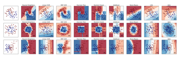
Project web site http://scikit-learn.org/stable/ for downloads, documentation, and tutorial.

There have been other tutorials making the rounds of various PyCon, SciPy, and PyData events over the last few years. They seem to be maturing. These were presented at SciPy 2013 by Olivier Grisel, Jake Vanderplas, and Gaël Varoquaux I like these for the coherence as a combined presentation. These people have done individual presentation at conferences too. This is a lot of video to watch split in to five sections. On YouTube:

Material for these including iPython notebooks are at Jake’s github page.

Also see Ben Lorica’s Six reasons why I recommend scikit-learn post on the O’Reilly site.

Lots of other conference videos of interest are at Vimeo’s PyData Portfolios.