Do You Speak Whale?

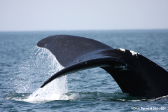
NARightWhaleTailToo cool, must learn more about this: Daniel Nouri’s Using deep learning to listen for whales uses multiple convolution layers to process inputs to a neural net. Details? Dunno much. In the whale case audio is treated as a greyscale image. Are the convolution layers treated as an independent feature generation stage in front of the neural net? Or are all weights learned together? Since convolution layer weights are shared among multiple neurons it seems a deep “normal” net could achieve similar results but may result in training times measured in archeological time units.

Good stuff in the references list at end of the post. Especially see the Nature article in [1] Computer science: The learning machines for an overview. Related: How Google Cracked House Number Identification in Street View and of course Kaggle’s The Marinexplore and Cornell University Whale Detection Challenge.

Cost Functions Series from Salford System

In the ten-part series How to Interpret Model Performance with Cost Functions Salford Systems continues to publish really well done data science tutorial webinars. Length of the segments vary with most about 10 to 20 minutes.

  • An Introduction to Understanding Cost Functions
  • Least Squares Deviation Cost for a Regression Problem
  • Least Absolute Deviation and Huber-M Cost for a Regression Problem
  • Introducing the Binary Classification Problem
  • Evaluating Prediction Success with Precision and Recall
  • Measuring Performance with the ROC Curve
  • Assessing Model Performance with Gains and Lift
  • Direct Interpretation of Response with Logistic Function
  • Multinomial Classification- Expected Cost
  • Multinomial Classification- Log Likelihood

MOOC Watch – January 2014

parallel programming iconA new crop of online courses has begun with the new year. To wrap my head around how GPU processing could be applied to Machine Learning and other Data Science areas I’ve enrolled in the University of Illinois’ Heterogeneous Parallel Programming via Coursera. This one started on January 6th. It began with Nvidia CUDA similar to how Udacity’s Intro to Parallel Programming is taught. The U-of-I class however plans to cover OpenCL and other interfaces after the groundwork is done with CUDA. I like this for avoiding potential vendor lock-in with CUDA only solutions.

statslearning logoOn January 21st StatLearning: Statistical Learning from Stanford University begins. They intend to cover all of An Introduction to Statistical Learning in nine weeks! This will be a lot wider in topics than Andrew Ng’s Machine Learning class but cannot possibly go as deep in that time. A pdf of the book will be available at no cost. The R language will be used but without a syllabus its not clear how heavy of a programming load comes with this class. The course will be on an open source version of the edX platform directly from Stanford. It is not through edx.org.

Udacity starts the year rolling out their New Course Experience and a Data Science track. The topics there are certainly interesting but I’m already max’d out with the two above. I am also wait-and-see on the New Course Experience. A quick look at what was available late last year using the new Udacity approach left me thinking the free-to-learn track may be pretty light weight. More depth in the form of projects and tutoring comes with a per course monthly fee. No more all-you-can-eat (can-learn) for free from Udacity.

scikit-learn info

scikit-learn-plots600

Project web site http://scikit-learn.org/stable/ for downloads, documentation, and tutorial.

There have been other tutorials making the rounds of various PyCon, SciPy, and PyData events over the last few years. They seem to be maturing. These were presented at SciPy 2013 by Olivier Grisel, Jake Vanderplas, and Gaël Varoquaux I like these for the coherence as a combined presentation. These people have done individual presentation at conferences too. This is a lot of video to watch split in to five sections. On YouTube:

Material for these including iPython notebooks are at Jake’s github page.

Also see Ben Lorica’s Six reasons why I recommend scikit-learn post on the O’Reilly site.

Lots of other conference videos of interest are at Vimeo’s PyData Portfolios.

Oh No! Machine Learning Class is Over

ShotPutFace
Wow! Andrew Ng’s Machine Learning Class via Coursera was amazing. What next? For more Andrew it looks like the iTunes store has two different versions of a 2008 on campus course. Access these via iTunesU > Universities & Colleges > Stanford > Engineering. Both seem to have the same 20 lecture videos.

This one ML-iTuneslooks like a newer reorganization of the material with topic titles interspersed among the videos. Where those topics lead is a mystery, they do not appear active on Win iTunes but might go somewhere on Apple hardware.

update: There is a much better organized version of this material at the stanford engineering everywhere site. Don’t bother with the iTunes version. This one has links to a syllabus, lecture videos and pdf’s, problem assignments and solutions, and other reference material.

Also online there is tutorial material on Unsupervised Feature Learning and Deep Learning which lists Andrew as the first contributor.

Lots of references from the Coursera Machine Learning wiki page ML:Useful Resources need to be explored too. You might need to be signed in on Coursera to access this page.

And finally there are two courses of interest on the Stanford Open Classroom site. Both Machine Learning and Unsupervised Feature Learning and Deep Learning have some interesting bits but neither seems to be complete. Works in progress? Or early MOOC efforts that won’t ever be finished?

Initial Results

Kaggle Digit Recognizer series

For this first attempt at getting actual Kaggle classification results the neural network from the Machine Learning course will only be changed in its input size dimension. A single hidden layer with 25 units is used. The default of 50 iterations for training and lambda of 1 for regularization will be used.

A little code rearrangement is in order here too. Some things in ex4.m aren’t needed (parts 2 through 5). Most of its remaining logic gets moved in to trainNN.m and a few lines are added to save the trained Theta matrices. New is runNN.m which loads Thetas, runs sample data through the network, and saves results in a Kaggle submission friendly format like so:

%% runNN.m

thetaFile = 'Thetas.mat';
testDataFile = 'test.mat';
resultsFile = 'results.csv';

% load trained model theta matrices
load(thetaFile);

% load test data
load(testDataFile);

% predict outputs from test samples
pred = predict(Theta1, Theta2, Xtest);

% change 10 labels back to 0 for Kaggle results
pred(pred==10) = 0;

% save predicted results
outfd = fopen(resultsFile, 'w');
fprintf(outfd, 'ImageId,Label\n');
for n = 1:size(pred)
	fprintf(outfd, '%d,%d\n', n, pred(n));
end
fclose(outfd);

Initial training of the net was done with all 42,000 samples. Splitting the data in to training and validation sets will be done later. After 50 training iterations the cost function value was 1.19. The network self-classified its training data with 87.698% accuracy. The initial Kaggle submission of the test data set achieved 86.600% accuracy, well behind the two Kaggle sample solutions with lots of room for improvement.

KdigitsSubmit-1

For an unguided attempt at improving on this result I trained a new network with 300 hidden nodes (still single layer) over 5000 iterations. Final self-classified accuracy was 100% and cost function was 0.0192. Run time for this was about 4200 seconds vs 10 seconds for the previous attempt. The Kaggle submission from this net was 92.629% accurate.

KdigitsSubmit-2

Adapting ML Class Code for Kaggle Data

Kaggle Digit Recognizer series

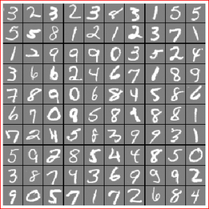
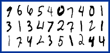
Sample data from the Machine Learning class is arranged as one sample per row with data values ranging from just a bit below 0 to a little above 1. Each digit image is a flattened 20×20 grey scale pixel array. The Kaggle data is arranged similarly but values range from 0 to 255. Kaggle digits are flattened 28×28 pixel arrays. The difference in value ranges should not be a problem for the exisiting code. The neural network input layer for Kaggle data will have 784 units vs the 400 used for the ML class data.

So the only code modification at this point is changing:

input_layer_size  = 400;  % 20x20 Input Images of Digits
hidden_layer_size = 25;   % 25 hidden units
num_labels = 10;          % 10 labels, from 1 to 10

to this:

input_layer_size  = 784;  % 28x28 Input Images of Digits
hidden_layer_size = 25;   % 25 hidden units
num_labels = 10;          % 10 labels, from 1 to 10

So we should be ready to go! The first thing we see running the top level Octave code is an image of a random selection of input samples.
KdigitsViz1
What? This can’t be right! Well it doesn’t really matter to the performance of classifying digit samples. But it is rather awkward to turn your head 90 degrees and look in a mirror at the computer display so lets fix this. The problem is caused by a difference of opinion on up/down/left/right for the two data sources. To fix this the displayData() function needs a change where the display_array is being accumulated. Change this:

        reshape(X(curr_ex, :), example_height, example_width) / max_val;

to this:

        reshape(X(curr_ex, :), example_height, example_width)' / max_val;

That’s it. Just transpose the result of reshape. A single character change.
KdigitsViz2
Much better.

Need Data

Kaggle Digit Recognizer series

Data for the digit recognizer is provided by Kaggle in csv formatted files. There are 42,000 training samples and 28,000 test samples. These can be read in to Octave with the csvread() function however this is painfully slow to witness. Much better to read the csv’s once and save the data in a more easily digestible binary format to speed up development and testing. I find it useful to have smaller slices of the data files available too. No need to throw 42,000 samples at the code when you’re just testing paths and logic. The code below reads the csv’s and saves full sized mat files along with 10%, 1%, and 0.1% slices.

%% training data set contains 42000 samples
%% the first row contains column labels

fname = 'train';
samples = csvread(strcat(fname, '.csv'));

samples = samples(2:end, :); % remove the first row (contains column labels)

rand('seed', 3.14159); % ensure this is repeatable
samples = samples(randperm(size(samples, 1)), :); % shuffle the sample order

X = samples(:, 2:end); % seperate inputs and outputs
y = samples(:, 1);

y(y==0) = 10; % change zero labels to tens to work with existing code

% save the full training data set
save('-float-binary', strcat(fname, '.mat'), 'X', 'y');

% save the abbreviated training data sets
sizes = [4200 420 42];
for s = sizes
    X = X(1:s, :);
    y = y(1:s, :);
    save('-float-binary', strcat(fname, int2str(s), '.mat'), 'X', 'y');
end

%% test data set contains 28000 samples
%% the first row contains column labels

fname = 'test';

Xtest = csvread(strcat(fname, '.csv'));

Xtest = Xtest(2:end, :); % remove the first row (contains column labels)

% save the full test data set
save('-float-binary', strcat(fname, '.mat'), 'Xtest');

% save the abbreviated test data sets
sizes = [2800 280 28];
for s = sizes
    Xtest = Xtest(1:s, :);
    save('-float-binary', strcat(fname, int2str(s), '.mat'), 'Xtest');
end

i.e. train.csv has been transmogrified in to train.mat, train4200.mat, train420.mat, and train42.mat.

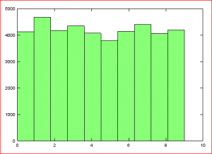
Just as a little sanity check lets have a look at how the training data target values are distributed. OK, not perfectly uniform, but a reasonable distribution of 0 through 9.
KdigitsHistogram

Performance Goal

Kaggle Digit Recognizer series

What is a good performance goal? If this problem were being started from scratch it would be reasonable to create a baseline classifier by a simple method such as counting each digit’s population in the training set and selecting the most abundant member as the  answer in all cases. In an evenly distributed population this would give an answer that was correct 10% of the time. It shouldn’t be too hard to beat that with a moderately more sophisticated classifier.

It’s not going to be that easy with this problem though. Kaggle has provided two sample solutions. First is a random forest which uses 1000 decision trees and votes on the digit identification. The other is a nearest-neighbor classifier that finds the 10 euclidean-closest trained samples and votes on its solution. These set the bar pretty high. The competition’s leader board shows them scoring 96.829% and 96.557% on test data submissions.